


PCA finance: introduction to the main linear technique for dimensionality reduction


June 18, 2026 8 min read 135 views
The Principal Component Analysis (PCA) algorithm identifies new perspectives (or axes) for datasets, making it more straightforward to segregate and cluster data instances. It generates as many axes as dimensions in a given dataset by design. However, these directions, known as Principal Components (PCs), are ranked based on their significance: the first PC captures the maximum possible data variance, the second one accounts for the second-largest variance, and so on. Once the initial data has been projected into this new subspace, we can eliminate some of the axes. This process reduces dimensionality while preserving most of the crucial information.
This article aims to demystify a fundamental technique used extensively in probability and statistics for dimensionality reduction factor analysis – PCA. Interestingly, PCA is not a dimensionality reduction method in the strictest sense, even though it is often portrayed as such. In reality, it modifies data specifically, preparing it for subsequent reduction.
How do you prepare data for Principal Component Analysis (PCA)?
PCA requires data standardization before calculating principal components. Standardization centers each variable around zero and scales it to a standard deviation of 1, preventing large-value features from dominating the analysis.
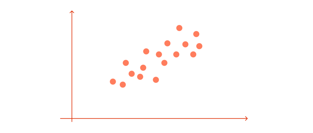
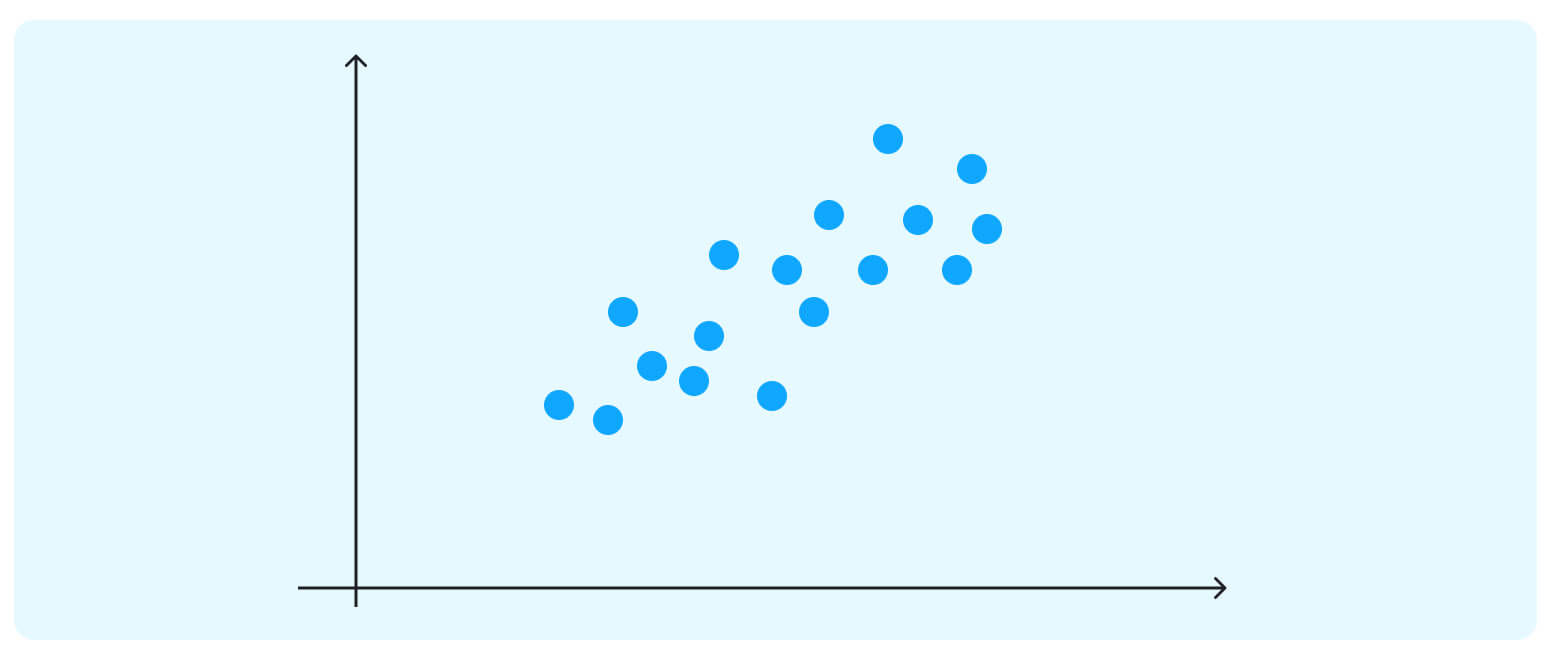
For example, suppose there are three variables – v1 in a 1-10 range, v2 in a 10-100 range, and v3 in a 100,000 to 1,000,000 range. Let us go ahead and compute an output using these original variables as predictors. We will get a heavily biased result because the third variable will disproportionately impact the output value. Before applying PCA, we must ensure that all our attributes (dimensions) are centered around zero and have a standard deviation 1. Now, we can calculate our first principal component. Imagine this is the dataset on which we are trying to do cluster analysis; we only have a data matrix with two dimensions.
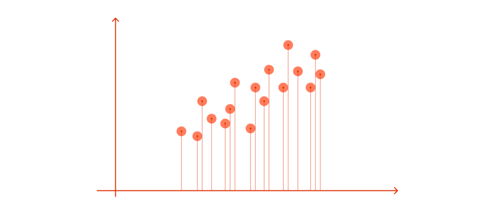
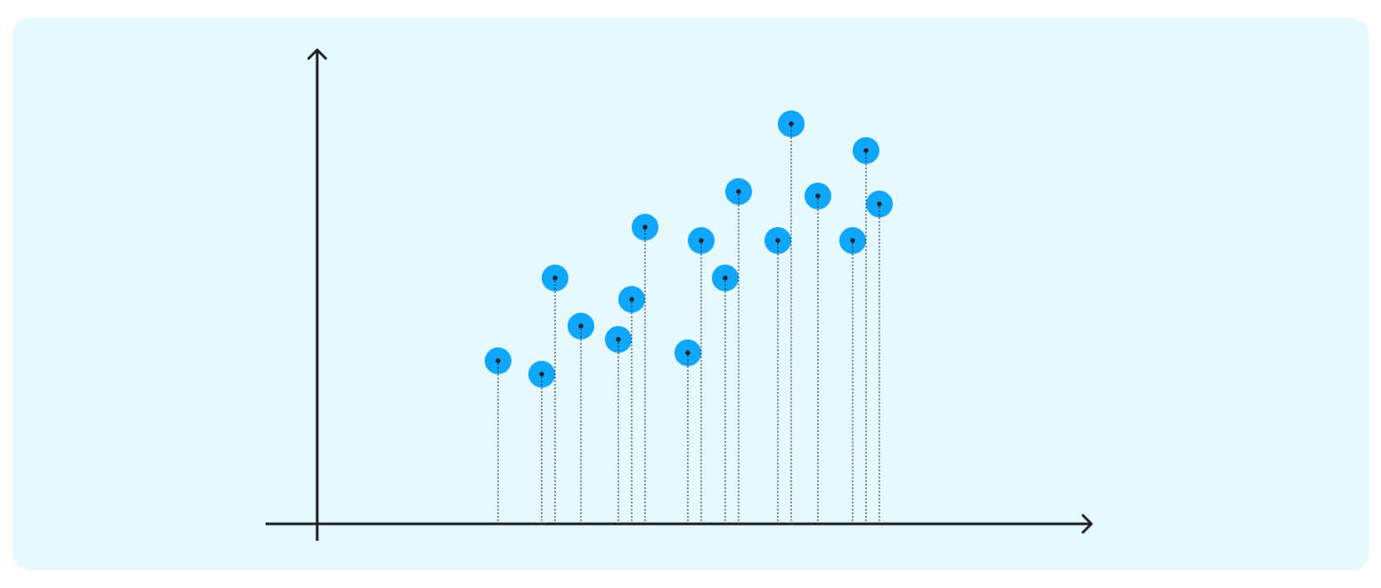
If we project the data onto the horizontal axis (our attribute 1), we will not see much spread; it will show a nearly equal distribution of the observations.
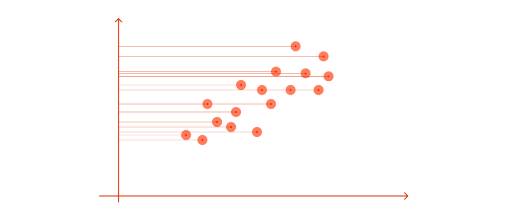
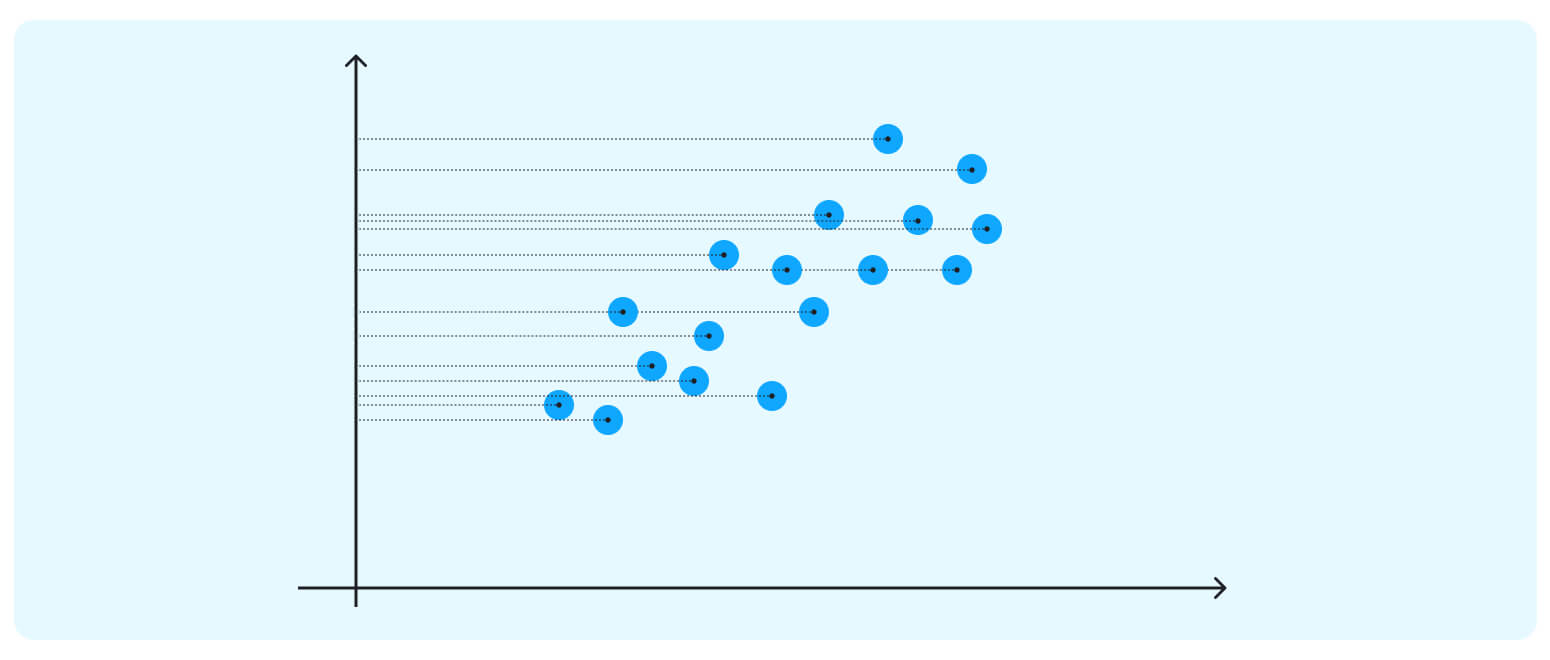
Attribute 2 could be more helpful too.
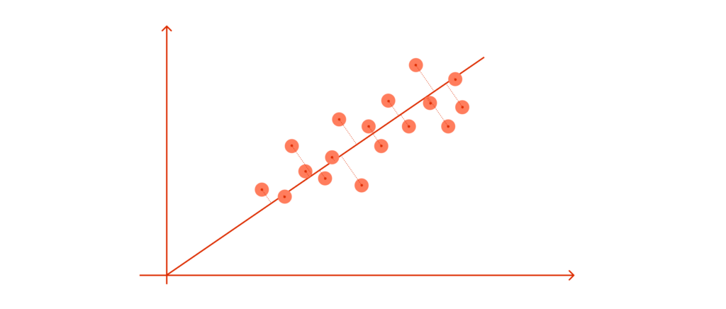
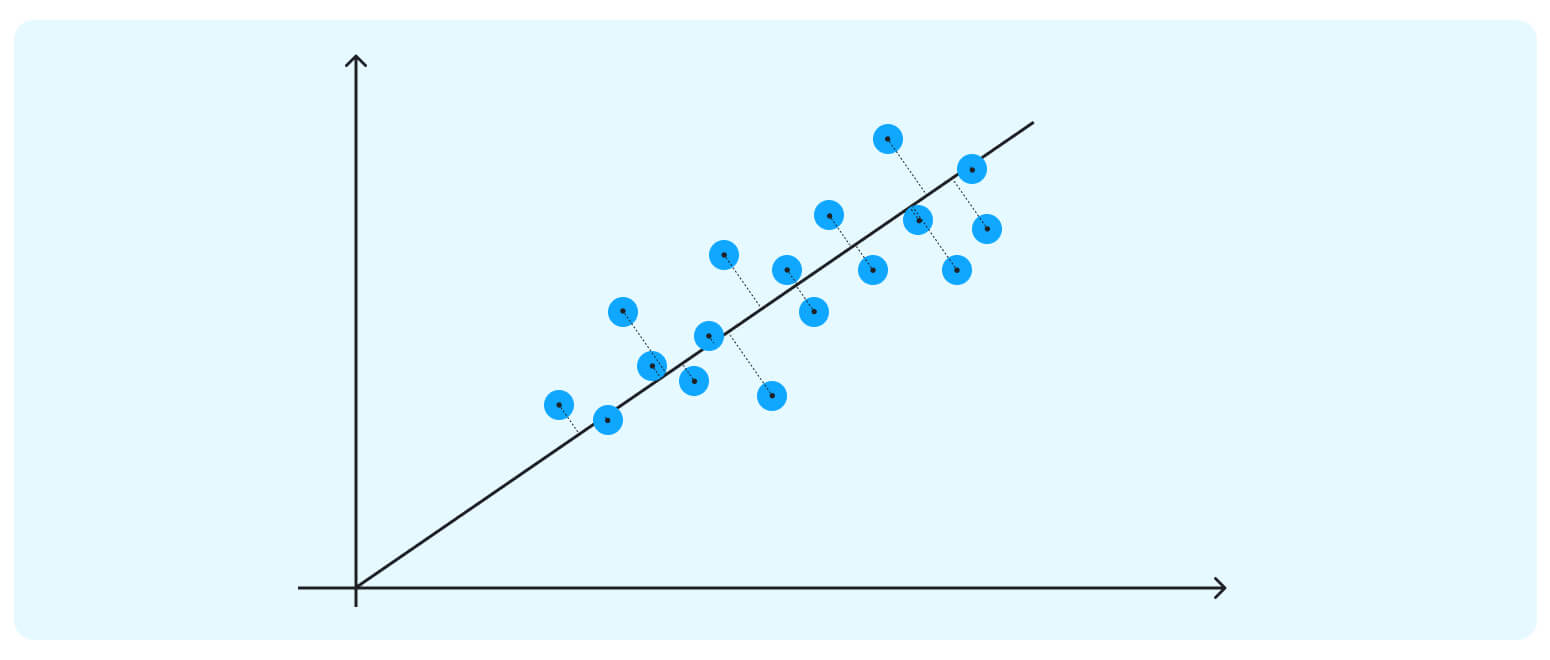
The data points in our case are spreading diagonally, so we need a new line to capture this better.

This axis is our first PC – a new direction (we can think of it as an attribute) that maximizes the total variance out of the whole data point (and thus, the clusters become much more apparent.) Besides maximizing the spread, this first PC sits through the direction of the data, minimizing the distances between all the points and the new axis.
The second PC must represent the second maximum amount of variance; it will be an orthogonal line to our first axis.
*Due to PCA’s math being based on eigenvectors and eigenvalues, new principal components will always come out orthogonal to the ones before them.
**Eigenvectors are vectors that are not knocked off their span by a linear transformation; they can hold on to their original direction while being stretched, shrunk, or reversed by linear combinations. Eigenvalues are factors by which these particular vectors are scaled.
How exactly do we calculate the first principal components (PC)?
To calculate the first principal component, start by finding the mean of each data column, then center the values by subtracting that mean. This prepares the dataset for covariance matrix calculation, which PCA uses to identify the directions with the most variance.
*Covariance is a statistical measure of an unnormalized effort that indicates the direction of the linear relationships between two (positive or negative) variables. A covariance matrix is a linear combination of a covariance calculated for a given matrix with covariance scores for every column with every other column.
Next, we utilize one of the methods for breaking up matrices (eigendecomposition or singular value decomposition) to turn our matrix into a list of eigenvectors that will define directions of axes in the new subspace and eigenvalues that will show the magnitude of those directions. We sort the vectors by their eigenvalues in decreasing order and thus get a ranking of the principal components.
That is it. Now we can ditch some dimensions and project our initial dataset into a reduced subspace without losing essential information about the original dataset. And since new axes capture the maximum variance in the original data, any clustering algorithm we will apply next will have an easier time grouping the data instances.
Why do financial analysts use PCA?
Financial analysts use PCA to reduce data complexity and identify the factors that drive market behavior. The technique transforms large sets of correlated variables into a smaller number of principal components, making financial models easier to analyze and interpret.
PCA is widely used in quantitative finance for portfolio construction, risk analysis, factor investing, and market forecasting. Data scientists also combine PCA with machine learning models to support time-series forecasting and financial data visualization.
Modern financial institutions process large volumes of market, economic, and company data. As the number of variables increases, identifying meaningful relationships becomes more difficult. PCA addresses this challenge by reducing correlated variables into a smaller set of factors that capture most of the information in the original dataset.
One of the most common applications of PCA in finance is portfolio risk analysis. By extracting the principal factors that explain market movements, analysts can evaluate risk exposures more effectively and simplify high-dimensional financial datasets. Research on portfolio risk analysis found that the first three principal components captured more than 75% of the variance in portfolio data, improving both risk assessment and portfolio optimization outcomes.
PCA also plays an important role in systemic risk modeling. Research published in Computational Economics introduced Principal Component Copulas, a framework that combines PCA with copula modeling to analyze tail dependence and systemic risk in high-dimensional financial markets. The authors found that the approach was effective at identifying market movements that increase systemic risk while supporting diversification analysis.
As financial datasets continue to grow in size and complexity, PCA remains one of the most widely used techniques for uncovering hidden market factors, reducing noise, and supporting more informed investment and risk-management decisions. Recent quantitative finance research continues to apply PCA to factor models, portfolio construction, and market analysis, demonstrating its ongoing relevance in modern financial modeling.
FAQ
Conclusion
PCA is a well-established technique for dimensionality reduction used to simplify complex datasets while preserving the most important patterns in the data. Data scientists apply it to high-dimensional data to improve clustering, support machine learning models, and make data analysis more efficient.
In finance, PCA helps identify key sources of risk and return by transforming correlated variables into a smaller set of uncorrelated principal components. This makes it easier to analyze portfolio risk, interpret market behavior, and work with large datasets that include asset prices, macroeconomic indicators, and other financial signals.
When applied correctly, PCA provides a structured way to reduce complexity without losing meaningful information, making it a practical tool for both financial analysis and broader data-driven decision-making.
Contact our experts for a free consultation to learn more about the algorithm and how your company can leverage its properties to achieve high-value business outcomes.


Your business results matter
Achieve them with minimized risk through our bespoke innovation capabilities. Fill in the form below.